3. Stokes class
Stokes is a class that manages Stokes vectors. It allows the user to create and manipulate them. The difference between Stokes and Jones formalisms is that Stokes vectors can handle partially polarized light, while Jones vectors can track the global phase of the electric field. However, Stokes objects store the global phase (if any) and use it when it is relevant.
3.1. Creating an instance
An instance must be created before starting to operate with the Stokes vector. The initialization accepts one argument: the name of the vector. This name will be used for printing:
[1]:
from py_pol.stokes import Stokes, create_Stokes, degrees
import numpy as np


S1 = Stokes("Source 1")
print(S1)
Source 1 is empty
Several Stokes objects can be created at the same time using the function create_Stokes.
[2]:
S2, S3 = create_Stokes(name=('Source 2', 'Source 3'))
print(S2, S3)

list_of_S = create_Stokes(N=3)
print(list_of_S)
Source 2 is empty
 Source 3 is empty

[S is empty
, S is empty
, S is empty
]
3.2. Stokes class fields
Stokes class objects have some fields where some methods and information stored:
M: 4xN array containing all the Stokes vectors.
name: Name of the object for print purposes.
size: Number of stored Stokes vectors.
shape: Shape desired for the outputs.
ndim: Number of dimensions for representation purposes.
type: Type of the object (‘Stokes’). This is used for determining the object class as using isinstance may throw unexpected results in .ipynb files.
Stokes class has two classes which groups different methods to extract information:
parameters: Object of class Parameters_Stokes.
checks: Object of class Checks_Stokes.
Analysis: Object of class Analysis_Stokes.
[3]:
E = Stokes("Source 1")
amp = np.random.rand(3,3)
E.linear_light(azimuth = 0, amplitude=amp)

print('Array: ', E.M)
print('Name: ', E.name)
print('Size: ', E.size)
print('Shape: ', E.shape)
print('Number of dimensions: ', E.ndim)
print('Type: ', E._type, '\n')

print('Parameters (intensity): \n', E.parameters.intensity(), '\n')
print('Checks (circularly polarized): \n', E.checks.is_circular(), '\n')
Array:  [[0.27783635 0.29282993 0.08162268 0.01928327 0.10014593 0.15666624
  0.72512106 0.42164197 0.03042108]
 [0.27783635 0.29282993 0.08162268 0.01928327 0.10014593 0.15666624
  0.72512106 0.42164197 0.03042108]
 [0.         0.         0.         0.         0.         0.
  0.         0.         0.        ]
 [0.         0.         0.         0.         0.         0.
  0.         0.         0.        ]]
Name:  Source 1
Size:  9
Shape:  [3, 3]
Number of dimensions:  2
Type:  Stokes

Parameters (intensity):
 [[0.27783635 0.29282993 0.08162268]
 [0.01928327 0.10014593 0.15666624]
 [0.72512106 0.42164197 0.03042108]]

Checks (circularly polarized):
 [[0. 0. 0.]
 [0. 0. 0.]
 [0. 0. 0.]]
3.3. Generating polarization states
As shown in the previous example, the Stokes matrix is initialized with all elements equal to zero. There are many methods that can be used to generate a more desirable vector:
from_components: Creates Stokes vectors directly from the 4 elements \(S_0\), \(S_1\), \(S_2\), \(S_3\).
from_matrix: Creates Stokes vectors from an external 4 x shape numpy array.
from_list: Creates a Jones_vector object directly from a list of 4 or 4x1 numpy arrays.
from_Jones: Creates Stokes vectors from a Jones_vector object.
linear_light: Creates Stokes vectors for pure linear polarizer light.
circular_light: Creates Stokes vectors for pure circular polarizer light.
elliptical_light Creates Stokes vectors for polarizer elliptical light.
general: Creates the most general Stokes vectors.
general_charac_angles Creates Stokes vectors given by their characteristic angles.
general_azimuth_ellipticity Creates Stokes vectors given by their azimuth and ellipticity.
For a more detailed description of each method, refer to the individual documentation of each one.
Example: Light linearly polarized.
[6]:
S1 = Stokes("Linear polarization")
S1.linear_light(azimuth=30*degrees)
print(S1)
Linear polarization =
[+1.000]
[+0.500]
[+0.866]
[+0.000]
The previous example only stores one Stokes vector. However, it is possible to store many Stokes vectors in the same object. This is useful specially when the same operation is performed upon all of them, as rotation. In this way, it is not required to use for loops, reducing significantly the computation time.
There are many ways of creating several Stokes vectors in the same object. The first way is creating an object with several identical vectors. This is performed using the length argument present in most creation methods:
[7]:
S = Stokes("Source 1")
S.linear_light(azimuth = 45*degrees, intensity=2, length = 5)
print(S)
Source 1 =
[+2.000]   [+2.000]   [+2.000]   [+2.000]   [+2.000]
[+0.000]   [+0.000]   [+0.000]   [+0.000]   [+0.000]
[+2.000]   [+2.000]   [+2.000]   [+2.000]   [+2.000]
[+0.000]   [+0.000]   [+0.000]   [+0.000]   [+0.000]
A second way of creating several vectors at the same time is using an array as one (or more) of the parameters of the creation methods. Take into account that, if you use this option, all parameters must have the same number of elements or just one element. Otherwise, the program will throw an exception.
[8]:
S = Stokes("Source 1")
angles = np.linspace(0, 90*degrees, 5)
S.linear_light(azimuth = angles, intensity=2)
print(S)
Source 1 =
[+2.000]   [+2.000]   [+2.000]   [+2.000]   [+2.000]
[+2.000]   [+1.414]   [+0.000]   [-1.414]   [-2.000]
[+0.000]   [+1.414]   [+2.000]   [+1.414]   [+0.000]
[+0.000]   [+0.000]   [+0.000]   [+0.000]   [+0.000]
If the parameters have dimension higher than 1, the program will store that information in order to make prints and plots. In that case, the print function separates the four components of the Stokes vectors:
[9]:
S = Stokes("Source 1")
I = np.random.rand(3,3)
S.linear_light(azimuth = 30*degrees, intensity=I)
print(S)
Source 1 S0 =
[[0.06238773 0.57797563 0.6247661 ]
 [0.48184591 0.09498877 0.59185975]
 [0.12173544 0.08507394 0.3738014 ]]
Source 1 S1 =
[[0.03119387 0.28898781 0.31238305]
 [0.24092296 0.04749438 0.29592987]
 [0.06086772 0.04253697 0.1869007 ]]
Source 1 S2 =
[[0.05402936 0.50054158 0.54106332]
 [0.4172908  0.08226268 0.51256558]
 [0.10542598 0.07367619 0.32372151]]
Source 1 S3 =
[[0. 0. 0.]
 [0. 0. 0.]
 [0. 0. 0.]]
3.3.1. Features of creation methods
Stokes formalism does not take into account the global phase of the light states. However, Stokes objects store it in the global_phase field. Use None if the global phase is unknown.
Most creation methods accept a global_phase argument that can be used to introduce it.
[10]:
S = Stokes("Source 1")
S.linear_light(azimuth = 45*degrees, global_phase=90*degrees)
print(S.global_phase / degrees)

S.remove_global_phase()
print(S.global_phase)
[90.]
0
Many creation methods accept an amplitude or an intensity parameter (\(a\) and \(b\) for elliptical_light) in order to set the electric field amplitude (the norm of the electric field vector) or the intensity. If both of them are given together to the method, it will use the amplitude:
[11]:
S = Stokes("Source 1")
S.linear_light(azimuth = 45*degrees, amplitude=5)
print(S)
_ = S.parameters.intensity(verbose=True)

S = Stokes("Source 2")
S.linear_light(azimuth = 45*degrees, intensity=2)
print(S)
_ = S.parameters.intensity(verbose=True)

S = Stokes("Source 3")
S.linear_light(azimuth = 45*degrees, intensity=2, amplitude=5)
print(S)
_ = S.parameters.intensity(verbose=True)
Source 1 =
[+25.000]
[+0.000]
[+25.000]
[+0.000]

The intensity of Source 1 is (a.u.):
25.0

Source 2 =
[+2.000]
[+0.000]
[+2.000]
[+0.000]

The intensity of Source 2 is (a.u.):
2.0

Source 3 =
[+25.000]
[+0.000]
[+25.000]
[+0.000]

The intensity of Source 3 is (a.u.):
25.0
Also, most creation methods accept two parameters: degree_pol and degree_depol, which represent the degrees of polarization and depolarization respectively. This allows creating partially polarized light states using the same methods.
Both degrees are complementary, so if both of them are given to the method, only degree_depol is used.
[12]:
S = Stokes("Source 1")
S.linear_light(azimuth = 45*degrees, intensity=5, degree_pol=0.8)
print(S)

S = Stokes("Source 2")
S.linear_light(azimuth = 45*degrees, intensity=5, degree_depol=0.8)
print(S)

S = Stokes("Source 3")
S.linear_light(azimuth = 45*degrees, intensity=5, degree_pol=0.8, degree_depol=0.8)
print(S)
Source 1 =
[+5.000]
[+0.000]
[+4.000]
[+0.000]

Source 2 =
[+5.000]
[+0.000]
[+3.000]
[+0.000]

Source 3 =
[+5.000]
[+0.000]
[+3.000]
[+0.000]
3.4. Basic operations
Some physical phenomena that affects polarized light are described by simple operations performed to their Stokes vectors.
3.4.1. Addition of two Stokes vectors
The interference of two light waves can be represented by the sum of their Stokes vectors. However, the global phase is important when two light states interfere, i.e., two vectors are added together. If both global phases are known (coherent sum), the polarized part of the Stokes vectors are transformed into Jones objects and added together. The result is tranformed back to a Stokes vector and the unpolarized parts are added.
[13]:
S1 = Stokes("Source 1")
S1.linear_light(azimuth = 0*degrees, amplitude=1, global_phase=0)
print(S1)
S2 = Stokes("Source 2")
S2.linear_light(azimuth = 0*degrees, amplitude=1, global_phase=90*degrees)
print(S2)
S3 = S1 + S2
print(S3)
Source 1 =
[+1.000]
[+1.000]
[+0.000]
[+0.000]

Source 2 =
[+1.000]
[+1.000]
[+0.000]
[+0.000]

Source 1 + Source 2 =
[+2.000]
[+2.000]
[+0.000]
[+0.000]
If one or both phases are unknown (they have a None value), the Stokes vectors are added directly (incoherent sum).
[14]:
S1 = Stokes("Source 1")
S1.linear_light(azimuth = 0*degrees, amplitude=1, global_phase=None)
print(S1)
S2 = Stokes("Source 2")
S2.linear_light(azimuth = 0*degrees, amplitude=1, global_phase=90*degrees)
print(S2)
S3 = S1 + S2
print(S3)
Source 1 =
[+1.000]
[+1.000]
[+0.000]
[+0.000]

Source 2 =
[+1.000]
[+1.000]
[+0.000]
[+0.000]

Source 1 + Source 2 =
[+2.000]
[+2.000]
[+0.000]
[+0.000]
3.4.2. Multiply by a constant
The absorption and gain experienced by a light wave is described by multiplying its Jones vector by a real positive number \(c\). The light wave will experience absorption if \(c<0\) and gain if \(c>0\):
[15]:
S1 = Stokes("Source 1")
S1.linear_light(azimuth = 0*degrees, amplitude = 0.5)
print(S1)

S2 = 2 * S1
print(S2)

S2 =  S1*3
print(S2)

S2 =  S1/3
print(S2)
Source 1 =
[+0.250]
[+0.250]
[+0.000]
[+0.000]

2 * Source 1 =
[+0.500]
[+0.500]
[+0.000]
[+0.000]

3 * Source 1 =
[+0.750]
[+0.750]
[+0.000]
[+0.000]

Source 1 / 3 =
[+0.083]
[+0.083]
[+0.000]
[+0.000]
If the constant is complex, the constant phase will be added to the global phase of the light, while its absolute value will increase or decrease the light intensity.
Take into account that real negative values are a special case of complex numbers whose phase is 180º.
[16]:
S1 = Stokes("Source 1")
S1.linear_light(azimuth = 0*degrees, intensity = 1)
print(S1)
_ = S1.parameters.global_phase(verbose=True)

c = 1j
S2 = c * S1
print(S2)
_ = S2.parameters.global_phase(verbose=True)

c = 0.5-0.5j
S2 = c * S1
print(S2)
_ = S2.parameters.global_phase(verbose=True)
Source 1 =
[+1.000]
[+1.000]
[+0.000]
[+0.000]

The global phase of Source 1 is (deg):
0.0

1j * Source 1 =
[+1.000]
[+1.000]
[+0.000]
[+0.000]

The global phase of 1j * Source 1 is (deg):
90.0

(0.5-0.5j) * Source 1 =
[+0.707]
[+0.707]
[+0.000]
[+0.000]

The global phase of (0.5-0.5j) * Source 1 is (deg):
-45.0
3.4.3. Equality
It is possible to compare two Stokes objects and tell if they are the same. It just compares the Stokes vectors and the global phase, not the rest of object fields.
[17]:
S1 = Stokes("Source 1")
S1.linear_light(azimuth = 0*degrees)
print(S1)
S2 = Stokes("Source 2")
angles = np.linspace(0, 90*degrees, 5)
S2.linear_light(azimuth = angles)
print(S2)
print('Comparison: ', S1==S2, '\n\n')

S1 = Stokes("Source 1")
S1.linear_light(azimuth = 0*degrees, global_phase=0)
print(S1)
S2 = Stokes("Source 2")
S2.linear_light(azimuth = 0*degrees, global_phase=0.01)
print(S2)
print('Comparison: ', S1==S2)
Source 1 =
[+1.000]
[+1.000]
[+0.000]
[+0.000]

Source 2 =
[+1.000]   [+1.000]   [+1.000]   [+1.000]   [+1.000]
[+1.000]   [+0.707]   [+0.000]   [-0.707]   [-1.000]
[+0.000]   [+0.707]   [+1.000]   [+0.707]   [+0.000]
[+0.000]   [+0.000]   [+0.000]   [+0.000]   [+0.000]

Source 1 - Source 2 =
[+0.000]   [+0.152]   [+0.586]   [+1.235]   [+2.000]
[+0.000]   [-0.141]   [-0.414]   [-0.472]   [-0.000]
[+0.000]   [-0.058]   [-0.414]   [-1.141]   [-2.000]
[+0.000]   [+0.000]   [+0.000]   [+0.000]   [+0.000]
 [0. 0. 0. 0. 0.]
Comparison:  [ True False False False False]


Source 1 =
[+1.000]
[+1.000]
[+0.000]
[+0.000]

Source 2 =
[+1.000]
[+1.000]
[+0.000]
[+0.000]

Source 1 - Source 2 =
[+0.000]
[+0.000]
[+0.000]
[+0.000]
 [0.]
Comparison:  [False]
3.4.4. Operations and multidimensionality
The basic operations of Stokes objects are subject to the same casting rules as numpy arrays. This means that they can be easily used even if one or both elements of the operation have more than one element.
Here are some examples:
[18]:
# Sum
S1 = Stokes("Source 1")
S1.linear_light(azimuth = 0*degrees, amplitude=1)
print(S1)
S2 = Stokes("Source 2")
angles = np.linspace(0, 90*degrees, 5)
S2.linear_light(azimuth = angles, amplitude=1, global_phase = 45*degrees)
print(S2)

S3 = S1 + S2
print(S3)
Source 1 =
[+1.000]
[+1.000]
[+0.000]
[+0.000]

Source 2 =
[+1.000]   [+1.000]   [+1.000]   [+1.000]   [+1.000]
[+1.000]   [+0.707]   [+0.000]   [-0.707]   [-1.000]
[+0.000]   [+0.707]   [+1.000]   [+0.707]   [+0.000]
[+0.000]   [+0.000]   [+0.000]   [+0.000]   [+0.000]

Source 1 + Source 2 =
[+3.414]   [+3.307]   [+3.000]   [+2.541]   [+2.000]
[+3.414]   [+3.014]   [+2.000]   [+0.834]   [+0.000]
[+0.000]   [+1.248]   [+2.000]   [+2.014]   [+1.414]
[+0.000]   [+0.541]   [+1.000]   [+1.307]   [+1.414]
[20]:
# Multply by a constant
S1 = Stokes("Source 1")
S1.linear_light(azimuth = 30*degrees, amplitude = 1)
print(S1)

c = np.linspace(0.1, 2.3, 5)
S2 = c * S1
print(S2)
Source 1 =
[+1.000]
[+0.500]
[+0.866]
[+0.000]

Source 1 =
[+0.100]   [+0.650]   [+1.200]   [+1.750]   [+2.300]
[+0.050]   [+0.325]   [+0.600]   [+0.875]   [+1.150]
[+0.087]   [+0.563]   [+1.039]   [+1.516]   [+1.992]
[+0.000]   [+0.000]   [+0.000]   [+0.000]   [+0.000]
3.5. Stokes vectors manipulation
There are several operations that can be applied to a Stokes vector. Some of them are common to all py_pol objects and are inherited from their parent Py_pol class:
clear: Removes data and name form Jones vector.
copy: Creates a copy of the Jones_vector object.
stretch: Stretches a Jones vector of size 1.
shape_like: Takes the shape of another object to use as its own.
reshape: Changes the shape of the object.
flatten: Transforms N-D objects into 1-D objects (0-D if only 1 element).
flip: Flips the object along some dimensions.
get_list: Creates a list with single elements.
from_list: Creates the object from a list of single elements.
concatenate: Canocatenates several objects into a single one.
draw: Draws the components of the object.
clear: Clears the information of the object.
The rest of the manipulation methods are:
simplify: Simplifies the Stokes vectors in several ways.
rotate: Rotates the Stokes vectors.
sum: Calculates the summatory of the Stokes vectors in the object.
reciprocal: Calculates the Stokes vectors that propagates backwards.
orthogonal: Calculates the orthogonal Stokes vectors.
normalize: Normalize the electric field to be normalized in electric field amplitude or intensity.
rotate_to_azimuth: Rotates the Stokes vectors to have a certain azimuth.
remove_global_phase: Calculates the global phase of the electric field (respect to the X component) and removes it.
add_global_phase: Adds a global phase to the Stokes vectors.
set_global_phase: Sets the global phase of the Stokes vectors.
set_depolarization: Sets the degree of depolarization.
add_depolarization: Increases the degree of depolarization.
For a more detailed description of each method, refer to the individual documentation of each one.
Example:
[21]:
S1 = Stokes('Source 1')
S1.linear_light(azimuth=0*degrees)
print(S1)

S1.rotate(angle=45*degrees)
print(S1)
Source 1 =
[+1.000]
[+1.000]
[+0.000]
[+0.000]

Source 1 @ 45.00 deg =
[+1.000]
[+0.000]
[+1.000]
[+0.000]
Most manipulation methods have the keep argument that specifies if the originial object must be preserved or transformed. If keep is True (default is False), a new object is created:
[22]:
S1 = Stokes('Source 1')
S1.linear_light(azimuth=0*degrees)

S2 = S1.rotate(angle=45*degrees, keep=True)
S2.name = 'Source 2'
print(S1, S2)

S2 = S1.rotate(angle=45*degrees, keep=False)
S2.name = 'Source 2'
print(S1, S2)
Source 1 =
[+1.000]
[+1.000]
[+0.000]
[+0.000]
 Source 2 =
[+1.000]
[+0.000]
[+1.000]
[+0.000]

Source 2 =
[+1.000]
[+0.000]
[+1.000]
[+0.000]
 Source 2 =
[+1.000]
[+0.000]
[+1.000]
[+0.000]
Stokes objects allow taking elements and changing them through indices like a numpy.ndarray.
Examples:
[23]:
M = np.random.rand(4, 3, 5)
S1 = Stokes('Original')
S1.from_matrix(M)
print(S1)

S2 = S1[0:3]
print(S2)
Original S0 =
[[0.73827998 0.3309537  0.42923983 0.20266855 0.97945782]
 [0.33310064 0.41272463 0.63421152 0.39573911 0.54567378]
 [0.04611144 0.77465159 0.03830944 0.74233396 0.21166797]]
Original S1 =
[[0.80725697 0.75942444 0.82534152 0.15295515 0.3583469 ]
 [0.90605304 0.94043943 0.41896632 0.0647273  0.16058601]
 [0.32477308 0.65895505 0.23844614 0.64100175 0.4681246 ]]
Original S2 =
[[0.82565326 0.46838908 0.07149297 0.51760866 0.8085559 ]
 [0.24613237 0.7992647  0.96896721 0.43505374 0.89333559]
 [0.79100309 0.43089529 0.08399607 0.987945   0.02170331]]
Original S3 =
[[0.02398912 0.69643331 0.04265789 0.68903845 0.32638138]
 [0.26542458 0.78317913 0.85479037 0.3183737  0.40564564]
 [0.07044742 0.27915799 0.50581986 0.21845827 0.49659919]]

Original_picked =
[+0.738]   [+0.331]   [+0.429]
[+0.807]   [+0.759]   [+0.825]
[+0.826]   [+0.468]   [+0.071]
[+0.024]   [+0.696]   [+0.043]
[24]:
S3.linear_light()
S4 = S1.copy()
S4.name = 'Cambiado'
S4[0:3,0:2] = S3
print(S4)
Cambiado S0 =
[[1.         1.         0.42923983 0.20266855 0.97945782]
 [1.         1.         0.63421152 0.39573911 0.54567378]
 [1.         1.         0.03830944 0.74233396 0.21166797]]
Cambiado S1 =
[[1.         1.         0.82534152 0.15295515 0.3583469 ]
 [1.         1.         0.41896632 0.0647273  0.16058601]
 [1.         1.         0.23844614 0.64100175 0.4681246 ]]
Cambiado S2 =
[[0.         0.         0.07149297 0.51760866 0.8085559 ]
 [0.         0.         0.96896721 0.43505374 0.89333559]
 [0.         0.         0.08399607 0.987945   0.02170331]]
Cambiado S3 =
[[0.         0.         0.04265789 0.68903845 0.32638138]
 [0.         0.         0.85479037 0.3183737  0.40564564]
 [0.         0.         0.50581986 0.21845827 0.49659919]]
3.5.1. Picking and setting
Py_pol objects allow taking elements and changing them through indices like a numpy.ndarray.
Examples:
[3]:
M = np.random.rand(4, 5)
S1 = Stokes('Original')
S1.from_matrix(M)
print(S1)

S2 = S1[1:3]
print(S2)
Original =
[+0.561]   [+0.450]   [+0.778]   [+0.601]   [+0.479]
[+0.695]   [+0.113]   [+0.805]   [+0.679]   [+0.663]
[+0.254]   [+0.415]   [+0.944]   [+0.003]   [+0.119]
[+0.217]   [+0.678]   [+0.093]   [+0.410]   [+0.767]

Original_picked =
[+0.450]   [+0.778]
[+0.113]   [+0.805]
[+0.415]   [+0.944]
[+0.678]   [+0.093]
[5]:
S1 = Stokes('Original')
angles = np.linspace(0,180*degrees, 25)
S1.linear_light(azimuth=angles, shape=[5,5])
print(S1)

S2 = S1[1:3,2:4]
print(S2)
Original S0 =
[[1. 1. 1. 1. 1.]
 [1. 1. 1. 1. 1.]
 [1. 1. 1. 1. 1.]
 [1. 1. 1. 1. 1.]
 [1. 1. 1. 1. 1.]]
Original S1 =
[[ 1.00000000e+00  9.65925826e-01  8.66025404e-01  7.07106781e-01
   5.00000000e-01]
 [ 2.58819045e-01  6.12323400e-17 -2.58819045e-01 -5.00000000e-01
  -7.07106781e-01]
 [-8.66025404e-01 -9.65925826e-01 -1.00000000e+00 -9.65925826e-01
  -8.66025404e-01]
 [-7.07106781e-01 -5.00000000e-01 -2.58819045e-01 -1.83697020e-16
   2.58819045e-01]
 [ 5.00000000e-01  7.07106781e-01  8.66025404e-01  9.65925826e-01
   1.00000000e+00]]
Original S2 =
[[ 0.00000000e+00  2.58819045e-01  5.00000000e-01  7.07106781e-01
   8.66025404e-01]
 [ 9.65925826e-01  1.00000000e+00  9.65925826e-01  8.66025404e-01
   7.07106781e-01]
 [ 5.00000000e-01  2.58819045e-01  1.22464680e-16 -2.58819045e-01
  -5.00000000e-01]
 [-7.07106781e-01 -8.66025404e-01 -9.65925826e-01 -1.00000000e+00
  -9.65925826e-01]
 [-8.66025404e-01 -7.07106781e-01 -5.00000000e-01 -2.58819045e-01
  -2.44929360e-16]]
Original S3 =
[[0. 0. 0. 0. 0.]
 [0. 0. 0. 0. 0.]
 [0. 0. 0. 0. 0.]
 [0. 0. 0. 0. 0.]
 [0. 0. 0. 0. 0.]]

Original_picked S0 =
[[1. 1.]
 [1. 1.]]
Original_picked S1 =
[[-0.25881905 -0.5       ]
 [-1.         -0.96592583]]
Original_picked S2 =
[[ 9.65925826e-01  8.66025404e-01]
 [ 1.22464680e-16 -2.58819045e-01]]
Original_picked S3 =
[[0. 0.]
 [0. 0.]]
3.5.2. Iterating
Py_pol objects are iterable. When introduced in a for loop, a new object picking in the first dimension is returned.
[6]:
angles = np.linspace(0, 180*degrees, 5)
Stotal = Stokes().general_azimuth_ellipticity(azimuth=angles, ellipticity=10*degrees)
for S in Stotal:
    print(S)
S_picked =
[+1.000]
[+0.940]
[+0.000]
[+0.342]

S_picked =
[+1.000]
[+0.000]
[+0.940]
[+0.342]

S_picked =
[+1.000]
[-0.940]
[+0.000]
[+0.342]

S_picked =
[+1.000]
[-0.000]
[-0.940]
[+0.342]

S_picked =
[+1.000]
[+0.940]
[+0.000]
[+0.342]
3.6. Parameters of Stokes vector
Several parameters can be measured from a Stokes vector. They are implemented in the independent class Parameters_Stokes_vector, which is stored in the parameters field of Stokes class.
components: Calculates the electric field components of the Stokes vectors.
amplitudes: Calculates the electric field amplitudes of the Stokes vectors.
intensity: Calculates the intensity of the Stokes vectors.
irradiance: Calculates the irradiance of the Stokes vectors.
alpha: Calculates the ratio between electric field amplitudes (\(E_x\)/\(E_y\)).
delay / delta: Calculates the delay (phase shift) between Ex and Ey components of the electric field.
charac_angles: Calculates both alpha and delay, the characteristic angles of the Stokes vectors.
azimuth: Calculates azimuth, that is, the orientation angle of the major axis.
ellipticity_angle: Calculates the ellipticity angle.
azimuth_ellipticity: Calculates both azimuth and ellipticity angles.
ellipse_axes: Calculates the length of major and minor axis (a,b).
ellipticity_param: Calculates the ellipticity parameter, b/a.
eccentricity: Calculates the eccentricity, the complementary of the ellipticity parameter.
global_phase: Calculates the global phase of the Stokes vectors (respect to the X component of the electric field).
degree_polarization: Calculates the degree of polarization of the Stokes vectors.
degree_depolarization: Calculates the degree of depolarization of the Stokes vectors.
degree_linear_polarization: Calculates the degree of linear polarization of the Stokes vectors.
degree_circular_polarization: Calculates the degree of circular polarization of the Stokes vectors.
norm: Calculates the norm of the Stokes vectors.
polarized_unpolarized: Divides the Stokes vector in Sp+Su, where Sp is fully-polarized and Su fully-unpolarized.
get_all: Returns a dictionary with all the parameters of Stokes vectors.
For a more detailed description of each method, refer to the individual documentation of each one.
Example:
[26]:
S = Stokes("Source 1")
S.linear_light(azimuth = 45*degrees)
I0 = S.parameters.intensity()
print(I0)
1.0
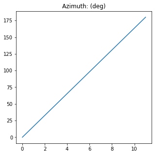
When several Stokes vectors are stored in the object, setting verbose argument to True makes the method print the values in screen. Also, 1D or 2D figures can be shown if the draw argument is set to True:
[28]:
az = np.linspace(0, 179.99*degrees, 12)
S = Stokes("Source 1")
S.general_azimuth_ellipticity(azimuth=az)
az = S.parameters.azimuth(draw=True, verbose=True)
The azimuth of Source 1 is (deg):
[  0.          16.36272727  32.72545455  49.08818182  65.45090909
  81.81363636  98.17636364 114.53909091 130.90181818 147.26454545
 163.62727273 179.99      ]
The mean value is 89.995 +- 56.484994071904
[29]:
az = np.linspace(0, 179.99*degrees, 128)
el = np.linspace(-45*degrees, 45*degrees, 128)
AZ, EL = np.meshgrid(az, el)

S = Stokes("Source 1")
S.general_azimuth_ellipticity(azimuth=AZ, ellipticity=EL)
AZ, EL = S.parameters.azimuth_ellipticity(draw=True, use_nan=False)
The azimuth of Source 1 is (deg):
The mean value is 88.58882812499999 +- 53.14074687799344

The ellipticity angle of Source 1 is (deg):
The mean value is 1.7763568394002505e-15 +- 26.184535918359188

There is a method in Parameters_Stokes class, get_all that computes all the parameters available and stores in a dictionary .dict_params(). Using the print function upon the Parameters_Stokes class invokes the method get_all.
Example:
[30]:
S1 = Stokes("Source 1")
S1. general_charac_angles(alpha=25*degrees,  delay=90*degrees,  intensity=1,    degree_pol=0.75)
print(S1,'\n')

print(S1.parameters)
Source 1 =
[+1.000]
[+0.482]
[+0.000]
[+0.575]


The intensity of Source 1 is (a.u.):
1.0
Low dimensionality, figure not available.

The elctric field amplitudes of Source 1 are (V/m):
  Ex (V/m)
0.7848855672213959
  Ey (V/m)
0.36599815077066683
  Eu (V/m)
0.4999999999999999
Low dimensionality, figure not available.

The global phase of Source 1 is (deg):
0.0
Low dimensionality, figure not available.

The degree of depolarization of Source 1 is:
0.6614378277661475
Low dimensionality, figure not available.

The degree of polarization of Source 1 is:
0.7500000000000001
Low dimensionality, figure not available.

The degree of linear polarization of Source 1 is:
0.48209070726490455
Low dimensionality, figure not available.

The degree of circular polarization of Source 1 is:
0.5745333323392335
Low dimensionality, figure not available.

The alpha of Source 1 is (deg):
25.000000000000004
Low dimensionality, figure not available.

The delay of Source 1 is (deg):
90.0
The mean value is 90.0 +- 0.0

The ellipticity parameter of Source 1 is:
0.4663076581549985
Low dimensionality, figure not available.

The ellipticity angle of Source 1 is (deg):
24.999999999999993
Low dimensionality, figure not available.

The azimuth of Source 1 is (deg):
2.090547128679534e-15
The mean value is 2.090547128679534e-15 +- 0.0

The eccentricity of Source 1 is:
0.8846226132911147
Low dimensionality, figure not available.

Polarized Source 1 =
[+0.750]
[+0.482]
[+0.000]
[+0.575]
 Unpolarized Source 1 =
[+0.250]
[+0.000]
[+0.000]
[+0.000]

The norm of Source 1 is (a.u.):
[1.25]
Low dimensionality, figure not available.
3.7. Checks of Stokes vectors
There are several checks that can be performed upon a Stokes vector. They are implemented in the independent class Checks_Stokes, which is stored in the checks field of Stokes class.
is_physical: Checks if the Stokes vectors are physically realizable.
is_linear: Checks if the Stokes vectors are lienarly polarized.
is_circular: Checks if the Stokes vectors are circularly polarized.
is_right_handed: Checks if the Stokes vectors rotation direction are right handed.
is_left_handed: Checks if the Stokes vectors rotation direction are left handed.
is_polarized: Checks if the Stokes vectors are at least partially polarized.
is_totally_polarized: Checks if the Stokes vectors are totally polarized.
is_depolarized: Checks if the Stokes vectors are at least partially depolarized.
is_totally_depolarized: Checks if the Stokes vectors are totally depolarized.
get_all: Returns a dictionary with all the checks of Stokes vectors.
For a more detailed description of each method, refer to the individual documentation of each one.
Example:
[31]:
S = Stokes("Source 1")
S.linear_light(azimuth = 45*degrees)
cond = S.checks.is_linear()
print(cond)
1.0
1D and 2D plot draws are also implemented for this class:
[32]:
alpha = np.linspace(30*degrees, 30*degrees, 128)
delay = np.linspace(0, 360*degrees, 128)
Alpha, Delay = np.meshgrid(alpha, delay)

S = Stokes("Source 1")
S.general_charac_angles(alpha=Alpha, delay=Delay)
_ = S.checks.is_right_handed(verbose=True, draw=True, use_nan=False)
Source 1 is right handed:
[[False False False ... False False False]
 [ True  True  True ...  True  True  True]
 [ True  True  True ...  True  True  True]
 ...
 [False False False ... False False False]
 [False False False ... False False False]
 [False False False ... False False False]]
The mean value is 0.4921875 +- 0.4999389611180049

3.8. Analysis of Stokes vectors
There there is one analysis that can be performed upon a Stokes vector. It is implemented in the independent class Analysis_Stokes, which is stored in the analysis field of Stokes class.
filter_physical_conditions: Forces the Stokes vectors to be physically realizable.
density: Calculates the density of states around the Poincaré sphere.
existence: Checks the existence of states around the Poincaré sphere.
For a more detailed description, refer to its documentation.
Example:
[33]:
S1 = Stokes("Source 1")
M = np.random.rand(4,6) * 2 - 1
S1.from_matrix(M)
print(S1)

S2 = S1.analysis.filter_physical_conditions(keep=True)
S2.name = 'Corrected source'
print(S2)
Source 1 =
[+0.682]   [+0.464]   [+0.949]   [+0.570]   [+0.642]   [+0.656]
[-0.982]   [-0.017]   [-0.486]   [-0.566]   [+0.171]   [+0.967]
[-0.155]   [-0.611]   [+0.300]   [+0.105]   [+0.824]   [+0.075]
[-0.665]   [-0.064]   [-0.691]   [-0.162]   [+0.257]   [-0.194]

Corrected source =
[+0.682]   [+0.464]   [+0.949]   [+0.570]   [+0.642]   [+0.656]
[-0.560]   [-0.013]   [-0.486]   [-0.540]   [+0.125]   [+0.642]
[-0.088]   [-0.461]   [+0.300]   [+0.100]   [+0.601]   [+0.050]
[-0.379]   [-0.048]   [-0.691]   [-0.154]   [+0.187]   [-0.129]